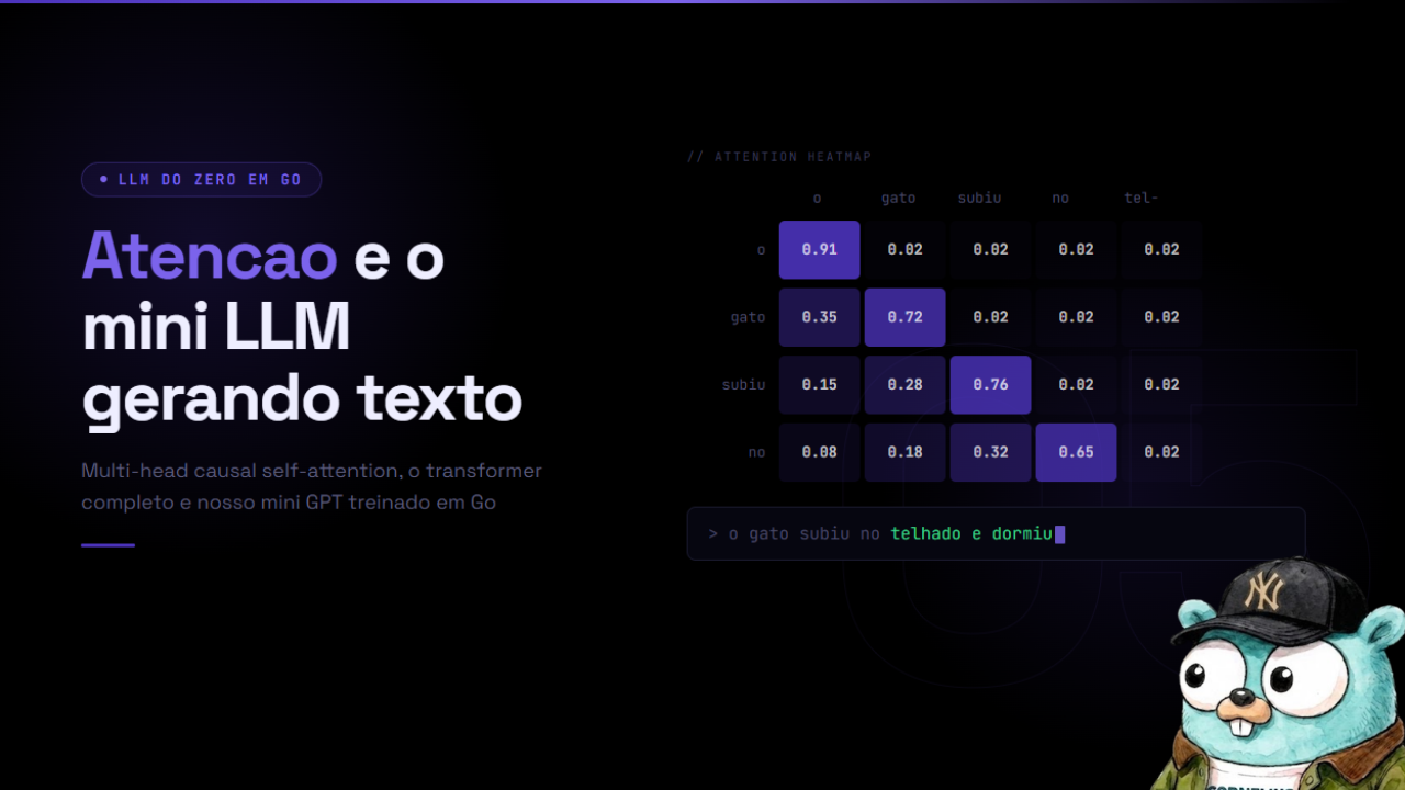
Attention and the mini LLM generating text

Hey everyone!

This is the fifth and final post in the LLM from Scratch in Go series. In the previous posts we built a BPE tokenizer (post 1), word vectors with semantic search (post 2), a Markov chain and its limits (post 3), and a feedforward network with manual backpropagation (post 4). This post covers videos 13 to 15 of the series.

We have arrived at the central mechanism that separates a transformer from everything that came before it: attention. This post implements multi-head causal self-attention in Go, assembles the full transformer block, builds the GPT model, and trains it to generate text.

The full code is at github.com/otavi/llm-do-zero.

---

The problem attention solves

The Markov chain from post 3 forgot everything beyond the last N tokens. The feedforward network from post 4 let each token run its own internal computations, but tokens could not see each other. Every position in the context was processed completely independently of all the others.

This creates a concrete problem. Consider the sentence:

The cat sat on the mat because it was comfortable.

The word “it” at position 9 needs to be resolved: what does it refer to? The cat or the mat? For a human it is obvious: cats get comfortable, mats usually do not. But for a model that processes each position independently, “it” has no way of knowing that the referent is at position 2.

Attention solves this. It lets position 9 (“it”) query all previous positions and learn which ones are relevant to it. After training, the “it” position learns to score the “cat” position highly and the “mat” position low, because the gradient pushed the weights in that direction every time the model got the context wrong.

This is not manually programmed logic. It is the gradient discovering, during training, which attention pattern minimizes prediction error.

---

Scaled dot-product attention

The attention mechanism starts with three learned matrices: Q (query), K (key), V (value). For each input token x, we compute:

Q = x · Wq
K = x · Wk
V = x · Wv

The idea is straightforward with a database analogy. Each token has:

• A query: what this token is looking for in the context
• A key: what this token is advertising to others
• A value: the content it provides when selected

The compatibility score between position i (query) and position j (key) is the dot product of their vectors:

score(i, j) = Q[i] · K[j]

We do this for all pairs, producing a T x T score matrix. Then we apply softmax to convert the scores into weights that sum to 1, and multiply by V to get a weighted sum of values:

Attention(Q, K, V) = softmax(Q · K^T / sqrt(d_k)) · V

The division by sqrt(d_k) is not cosmetic. Without it, when d_k is large, the dot products become very large in magnitude, which pushes the softmax into near-zero gradient regions (the curve saturates). The division keeps scores at a scale where gradients flow well during training.

A minimal worked example: 3 tokens, vectors of dimension 4.

Suppose after computing Q and K we have (for a single head):

Q = [[0.1, 0.8, 0.2, 0.5],   # token 0
     [0.3, 0.1, 0.9, 0.2],   # token 1
     [0.7, 0.4, 0.1, 0.6]]   # token 2

K = [[0.2, 0.7, 0.3, 0.4],
     [0.5, 0.2, 0.8, 0.1],
     [0.6, 0.9, 0.2, 0.3]]

The raw score between token 2 (query) and token 0 (key):

dot = 0.7*0.2 + 0.4*0.7 + 0.1*0.3 + 0.6*0.4 = 0.14 + 0.28 + 0.03 + 0.24 = 0.69
score = 0.69 / sqrt(4) = 0.69 / 2.0 = 0.345

We do this for each pair (i, j) where j <= i (with the causal mask, covered next), apply softmax to the row, and get the attention weights of token 2 over tokens 0 and 1.

---

Causal masking

For text generation, the model cannot attend to future positions. When we are at position i, tokens i+1, i+2, ... have not been generated yet. If the model could look at them during training, it would copy from the answer key and learn nothing useful.

The fix is the causal mask: before applying softmax, we set scores for j > i to negative infinity. The softmax of negative infinity is 0, so those positions contribute nothing to the weighted sum.

In the project code, this appears directly in the forward loop:

for j := 0; j <= i; j++ {  // causal: j <= i only
    var dot float64
    for d := 0; d < Dh; d++ {
        dot += q.At(i, h*Dh+d) * k.At(j, h*Dh+d)
    }
    score := dot * mha.scale
    row[j] = score
    if score > maxVal { maxVal = score }
}

The inner loop runs from j = 0 to j = i inclusive. Positions j > i never receive a score – they simply do not exist in the computation. The effect is identical to applying a negative infinity mask before softmax, but more efficient because it avoids computing scores that would be discarded.

This is the “causal” in “causal self-attention.” Language models use causal attention. Encoding models (like BERT) use bidirectional attention where all tokens can attend to all others.

---

Multi-head attention

Instead of one large attention over the full dimension D, we split into H smaller heads, each with dimension Dh = D / H. Each head runs its own independent attention and the results are concatenated.

Why does this work better? Because each head can specialize in different patterns. One head might learn syntactic dependencies (subject-verb), another might learn semantic references (pronoun-antecedent), another might focus on relative position patterns. With a single large attention, the model would have to resolve all those patterns with the same weights.

In the project code at internal/model/attention.go:

func NewMultiHeadAttention(cfg Config) *MultiHeadAttention {
    D := cfg.EmbedDim
    mha := &MultiHeadAttention{
        Wq:       tensor.New(D, D),
        Wk:       tensor.New(D, D),
        Wv:       tensor.New(D, D),
        Wo:       tensor.New(D, D),
        numHeads: cfg.NumHeads,
        headDim:  D / cfg.NumHeads,
        scale:    1.0 / math.Sqrt(float64(D/cfg.NumHeads)),
    }
    const std = 0.02
    mha.Wq.RandNormal(0, std)
    mha.Wk.RandNormal(0, std)
    mha.Wv.RandNormal(0, std)
    mha.Wo.RandNormal(0, std)
    return mha
}

Four learned matrices: Wq, Wk, Wv (each D x D), and Wo (the output projection, also D x D). Initialization with standard deviation 0.02 follows the GPT-2 convention – keeps weights small enough that residual connections dominate at the start of training.

In the forward pass, heads are processed in a loop (in production this would be a batched matrix operation):

func (mha *MultiHeadAttention) Forward(x *tensor.Tensor) *tensor.Tensor {
    T, D := x.Rows, x.Cols
    H, Dh := mha.numHeads, mha.headDim

    q := tensor.MatMul(x, mha.Wq)
    k := tensor.MatMul(x, mha.Wk)
    v := tensor.MatMul(x, mha.Wv)

    attn := make([][]float64, H*T)
    for row := range attn {
        attn[row] = make([]float64, T)
    }
    ctx := tensor.New(T, D)

    for h := 0; h < H; h++ {
        for i := 0; i < T; i++ {
            row := attn[h*T+i]
            var maxVal float64 = math.Inf(-1)
            for j := 0; j <= i; j++ {
                var dot float64
                for d := 0; d < Dh; d++ {
                    dot += q.At(i, h*Dh+d) * k.At(j, h*Dh+d)
                }
                score := dot * mha.scale
                row[j] = score
                if score > maxVal { maxVal = score }
            }
            var sum float64
            for j := 0; j <= i; j++ {
                e := math.Exp(row[j] - maxVal)
                row[j] = e
                sum += e
            }
            for j := 0; j <= i; j++ { row[j] /= sum }

            for d := 0; d < Dh; d++ {
                var weighted float64
                for j := 0; j <= i; j++ {
                    weighted += row[j] * v.At(j, h*Dh+d)
                }
                ctx.Set(i, h*Dh+d, weighted)
            }
        }
    }
    mha.cache.x, mha.cache.q, mha.cache.k = x, q, k
    mha.cache.v, mha.cache.attn, mha.cache.ctx = v, attn, ctx
    return tensor.MatMul(ctx, mha.Wo)
}

The access q.At(i, h*Dh+d) extracts the dimension slice [h*Dh : (h+1)*Dh] of the query vector at token i, corresponding to head h. The heads are interleaved in the same matrix rather than stored as separate tensors – this is more memory-efficient and easier to implement with simple matrix multiplication.

The row[j] - maxVal trick in the softmax is the numerically stable softmax: instead of computing exp(x) directly (which can overflow), subtract the maximum first. The mathematical result is identical because maxVal cancels in the denominator.

After accumulating weighted context across H heads, the result passes through the Wo matrix, which mixes the information from all heads back into the original D-dimensional space.

---

The full transformer block

Attention alone is not the transformer. The transformer block combines attention, feedforward, and two structural patterns that make training deep networks feasible: residual connections and layer normalization.

The code in internal/model/block.go:

// Block: x1 = x + Attn(LN1(x))
//        out = x1 + FFN(LN2(x1))
type Block struct {
    Ln1  *LayerNorm
    Attn *MultiHeadAttention
    Ln2  *LayerNorm
    FFN  *FeedForward
}

func (b *Block) Forward(x *tensor.Tensor) *tensor.Tensor {
    ln1Out := b.Ln1.Forward(x)
    attnOut := b.Attn.Forward(ln1Out)
    x1 := tensor.Add(x, attnOut)      // residual connection

    ln2Out := b.Ln2.Forward(x1)
    ffnOut := b.FFN.Forward(ln2Out)
    return tensor.Add(x1, ffnOut)     // residual connection
}

Residual connections (x + sublayer(x)): the original signal is added to the output of each sublayer. Why does this matter? During backpropagation, the gradient flows through the addition. The derivative of f(x) + x with respect to x is f'(x) + 1. The +1 guarantees the gradient never fully vanishes – it can always pass straight through the residual connection without needing to traverse the sublayer. Without residuals, networks with dozens of layers suffer from the vanishing gradient problem.

Pre-norm vs post-norm: our code applies LayerNorm before each sublayer (b.Ln1.Forward(x) before b.Attn.Forward(...)). The original “Attention Is All You Need” paper used post-norm (normalize after). Pre-norm became the standard because it produces more stable training, especially for large models. With pre-norm, residuals arrive un-normalized directly at the addition, which preserves gradient scale.

LayerNorm: normalizes each token vector independently (zero mean, unit variance), then applies learned scale and bias. Unlike BatchNorm, LayerNorm does not depend on batch size, which matters for inference with batch size 1.

FeedForward: the network from post 4. For each position, applies two linear layers with an activation in between: FFN(x) = GELU(x·W1 + b1)·W2 + b2. With FFNDim = 4*EmbedDim, the feedforward has 4x more parameters than the attention matrices. This is where the model stores “facts” about the world – attention routes information, the feedforward processes and transforms it.

---

The full GPT model

With the blocks in place, the GPT model in internal/model/gpt.go is straightforward:

// GPT: input ids -> Embedding (token + position) -> N x Block -> LayerNorm -> Linear head -> logits
type GPT struct {
    Embed  *Embedding
    Blocks []*Block
    LnF    *LayerNorm
    Head   *tensor.Tensor
    cfg    Config
}

func (g *GPT) Forward(ids []int) *tensor.Tensor {
    x := g.Embed.Forward(ids)
    for _, block := range g.Blocks {
        x = block.Forward(x)
    }
    x = g.LnF.Forward(x)
    return tensor.MatMul(x, g.Head)
}

Step by step:

1. Embedding: each token ID is mapped to a vector of dimension EmbedDim. But the transformer has no intrinsic sense of order – attention does not know whether a token is at position 0 or position 50. So we add a second vector: the positional embedding. Each position 0..ContextLen has its own learned vector. The final input to the blocks is token_embedding[id] + position_embedding[pos].

2. N transformer blocks in sequence: each block receives a T x D tensor and returns a T x D tensor of the same shape. The number of blocks NumLayers controls the depth of the model. Deeper layers learn more abstract representations.

3. Final LayerNorm (LnF): normalizes the representations before projecting to the vocabulary.

4. Linear head: projects from EmbedDim to VocabSize. The result is logits – a score for each vocabulary token at each position. We do not apply softmax here; that is done during the loss computation (cross-entropy over logits is more numerically stable) or during generation (where we divide by temperature before softmax).

The training objective is: for each position t, token ids[t+1] should have the highest logit. The model learns to predict the next token at every position simultaneously – this is why transformers are so efficient to train.

How many parameters does TinyConfig have?

var TinyConfig = Config{
    VocabSize:  256,
    ContextLen: 128,
    EmbedDim:   64,
    NumHeads:   4,
    NumLayers:  2,
    FFNDim:     256,
}

Counting:

Component	Calculation	Parameters
Token embedding	256 x 64	16,384
Positional embedding	128 x 64	8,192
Attention (Wq+Wk+Wv+Wo) per block	4 x 64 x 64	16,384
FFN (W1+b1+W2+b2) per block	64x256 + 256 + 256x64 + 64	33,088
LayerNorm (2 per block)	4 x 64 x 2	512
Final LayerNorm	64 x 2	128
Linear head	64 x 256	16,384
2 blocks total	2 x (16,384 + 33,088 + 512)	99,968
Total		~141,000

Around 141 thousand parameters. For comparison: GPT-2 small has 117 million. GPT-3 has 175 billion. GPT-4 is estimated at hundreds of billions. The architecture is identical – what changes is scale.

---

Autoregressive text generation

The Generate function in gpt.go implements token-by-token generation:

func (g *GPT) Generate(prompt []int, maxNew int, temperature float64) []int {
    ids := make([]int, len(prompt))
    copy(ids, prompt)
    for range maxNew {
        ctx := ids
        if len(ctx) > g.cfg.ContextLen {
            ctx = ctx[len(ctx)-g.cfg.ContextLen:]
        }
        logits := g.Forward(ctx)
        next := sampleLogits(logits.Row(len(ctx)-1), temperature)
        ids = append(ids, next)
    }
    return ids[len(prompt):]
}

The key point: logits.Row(len(ctx)-1) extracts only the last row of the logits. The model produces logits for all positions, but we only care about the last position to decide the next token. The other positions are used only during training to compute the loss in parallel.

If the context accumulates more than ContextLen tokens, we truncate from the beginning, always keeping the most recent tokens. The model has no memory beyond its context window.

---

Temperature and sampling

The sampleLogits function controls how we choose the next token from the logits:

p_i = exp((logit_i - max_logit) / temperature) / sum_j(exp((logit_j - max_logit) / temperature))

Temperature 1.0 is standard softmax – probabilities faithfully reflect what the model learned. Temperature 0 (in the limit) is greedy – always picks the highest logit, no randomness. Temperature > 1 flattens the distribution, making unlikely tokens more probable – the text becomes more creative and less coherent. Temperature < 1 sharpens the distribution, concentrating probability on the most likely token – the text becomes more deterministic and repetitive.

For practical applications:

• Creative writing (prose, poetry): 0.7 to 1.0
• Code completion: 0.2 to 0.4
• Information extraction / factual answers: 0.1 to 0.3
• Brainstorming / exploration: 1.0 to 1.2

Temperature too high produces text that does not make sense. Temperature too low produces text that gets stuck in repetitive loops. The range 0.7-0.9 is a good starting point for most natural text generation.

---

Training and generating text

The training loop in internal/train/trainer.go:

func (t *Trainer) Train() {
    params := t.Model.Parameters()
    for step := range t.Cfg.MaxSteps {
        inputs, targets := t.Dataset.Batch(t.Cfg.BatchSize, seqLen)
        t.Model.ZeroGrad()
        var totalLoss float64
        scale := 1.0 / float64(t.Cfg.BatchSize)
        for b := range t.Cfg.BatchSize {
            logits := t.Model.Forward(inputs[b])
            loss, dLogits := crossEntropy(logits, targets[b])
            totalLoss += loss
            for i := range dLogits.Data { dLogits.Data[i] *= scale }
            t.Model.Backward(dLogits)
        }
        t.Optim.Step(params)
        if step%t.Cfg.LogEvery == 0 {
            avg := totalLoss / float64(t.Cfg.BatchSize)
            fmt.Printf("step %6d | loss %.4f | ppl %.2f\n", step, avg, math.Exp(avg))
        }
    }
}

For each step: grab a batch of (input, target) pairs, zero the gradients, run forward and backward on each sequence in the batch, accumulate gradients, then update the parameters. The scale = 1/BatchSize normalizes the gradient so the learning rate does not need to be adjusted as batch size changes.

Perplexity (ppl = exp(loss)) is the intuitive metric: perplexity 255 means the model is equally confused about 255 possible tokens (at the start, with a 256-byte vocabulary, this makes sense). Perplexity 6-8 means the model is effectively choosing between 6-8 reasonable options.

To train in practice:

# Clone the project
git clone https://github.com/otavi/llm-do-zero
cd llm-do-zero

# Add training text (Shakespeare, news articles, code, anything)
# Place it in data/train.txt

# Train
go run ./cmd/train

Expected output during training:

step      0 | loss 5.5450 | ppl 255.75
step    500 | loss 3.2100 | ppl 24.76
step   1000 | loss 2.8400 | ppl 17.12
step   5000 | loss 2.1200 | ppl 8.33
step  10000 | loss 1.8900 | ppl 6.62

The drop in perplexity from 255 to 6 shows the model learning the structure of the text.

# Generate text
go run ./cmd/generate --prompt "The king" --tokens 100 --temperature 0.8

After training on Shakespeare, the output looks something like this:

The king hath spoken well of thee,
And bid me come to court before the sun
Doth rise upon the castle. I have told
My lord the matter, yet he speaks of war
And will not hear the counsel of his men.

It is not perfect. Every 10-15 words the text starts to drift. But the metrical structure, the archaic vocabulary, and the grammatical constructions are clearly Shakespearean. The model learned the patterns of the training text.

---

Limitations of our mini GPT

Let us be honest about what we built.

Our TinyConfig has roughly 141 thousand parameters trained on a few MB of text. GPT-2 small has 117 million parameters. GPT-3 has 175 billion. GPT-4 is estimated at hundreds of billions. The scale difference is 3 to 6 orders of magnitude.

What this means in practice:

• Generated text is coherent within 5-15 tokens, then degrades
• The model cannot “memorize facts” – too few parameters for the data it would need
• The 128-token context window is small (GPT-4 works with 128k tokens)
• Training on CPU can take hours to get reasonable results

What our model gets right:

• The architecture is identical to the original GPT
• Every component that matters is implemented: tokenization, embeddings, causal multi-head attention, transformer blocks, layer norm, residuals, autoregressive generation
• The code is explicit about every step – no magic hidden in framework abstractions

The difference between our mini GPT and ChatGPT is scale, training data, and RLHF fine-tuning. The central architecture is the same one Vaswani et al. published in 2017.

One detail our implementation omits for simplicity: in production, the backward pass through the transformer requires implementing gradients for MatMul, softmax, LayerNorm, and attention itself. Our code runs the correct forward pass, and the backward structure follows the same pattern as post 4 (gradient flowing backward through the chain of operations). For a complete educational backward implementation, the repository has the details.

---

Series conclusion

This series walked the path from strings.Split(text, " ") to a working GPT in Go, without any external machine learning library.

Post 1 - Tokenization: turned text into integer sequences. Implemented UTF-8, byte vocabulary, and the BPE algorithm that compresses frequent sequences into single tokens. Without tokenization, the model has no input.

Post 2 - Word vectors: turned tokens into dense vectors of dimension EmbedDim. Implemented semantic search and saw that words with related meanings end up close in vector space. Without embeddings, the model has no representation.

Post 3 - Markov chain: the first predictive model. Learned transition probabilities between tokens and generated text from them. The limit became clear: the context window is rigid and the model has no parameters to learn internal representations.

Post 4 - Feedforward network and backpropagation: implemented the first neural network with manual gradient descent. Each token passes through non-linear transformations and the model learns from its mistakes. The limit was explicit: tokens do not communicate.

Post 5 - Attention and the transformer: tokens finally see each other. Each position can query all previous ones and decide which are relevant. Multi-head attention, transformer blocks with residuals, and the full GPT with autoregressive generation.

The full code is at github.com/otavi/llm-do-zero. Each component has its own package, tests cover the main cases, and the train and generate commands work with any text file.

If you got here, you understand the fundamentals of how a transformer works. Not at the level of “I read an article about this,” but at the level of “I wrote every operation line by line and watched the gradients descend.” That matters.

---

References

• Vaswani, A. et al. “Attention Is All You Need” (2017) - arxiv.org/abs/1706.03762
• Radford, A. et al. “Language Models are Unsupervised Multitask Learners” (GPT-2, 2019) - openai.com/research/language-unsupervised
• Karpathy, A. nanoGPT - github.com/karpathy/nanoGPT
• Alammar, J. “The Illustrated Transformer” - jalammar.github.io/illustrated-transformer/
• Rush, A. “The Annotated Transformer” - nlp.seas.harvard.edu/annotated-transformer/
• Geva, M. et al. “Transformer Feed-Forward Layers Are Key-Value Memories” (2021) - arxiv.org/abs/2012.14913